The Bullwhip (Forrester) Effect: How Small and Periodic Fluctuations in Customer Demand Can Have a Drastic Impact on a Supply Chain.
The Bullwhip Effect is a fairly simple and straightforward concept. It outlines how a periodic change in customer demand can have substantial impacts on inventory counts within a given supply chain.
Jay Forrester’s “Industrial Dynamics”, written in 1961, was the first source to outline how an increase in consumer/end-user demand can directly impact the inventory levels and inventory costs of every player within a supply chain. Understanding the Bullwhip Effect is the easy part; eliminating the effect as a going concern is something else entirely. So, how does the Forrester Effect take hold and what can companies do, if anything, to better anticipate these aforementioned sudden spikes and dips in customer demand.
The Forrester Effect
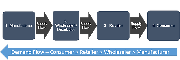
Let’s take an example of a consumer-based product and how the Forrester Effect might impact the inventory counts for every company within the supply chain. First, there is the manufacturer. The manufacturer produces a finished good. Their production throughput is based upon the projected sales volumes originating from a wholesaler/distributor. The wholesaler/distributor distributes the product on behalf of the manufacturer. The wholesaler’s forecast is based upon projected sales from a retailer.
The retailer is the customer-facing sales company that provides the finished good directly to the consumer. They base their inventory counts and subsequent sales forecasts directly from what the customer buys, how much they buy, and most importantly, when they buy. If demand increases from the consumer, then that demand flows back through the supply chain from the retailer to the wholesaler/distributor and finally back to the manufacturer. This supply chain is outlined below.
The BullWhip Effect defines what happens when demand from consumers suddenly, and quite unexpectedly, spikes upwards. In this case, consumers suddenly purchase way more than anticipated and the resulting increase in consumer demand forces the supply chain to adjust inventory counts accordingly. An increase in customer demand means the retailer will increase their order size to the wholesaler, who will in turn increase their order size to the manufacturer. Finally, the manufacturer will see this increase demand and purchase more raw materials for production in order to keep up with the forecasted increase emerging down the supply chain.
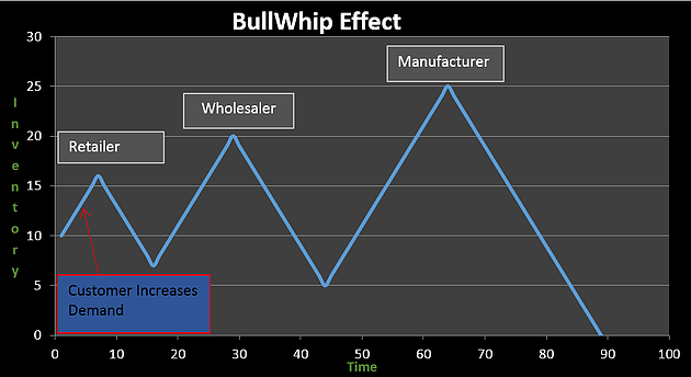
The following graph illustrates how the Bullwhip Effect would work. The consumer unexpectedly increases demand and that demand empties out the shelves within the retailer. That sudden increase in orders means the retailer will need to replenish their shelves. They anticipate seeing the same high level of customer demand and order accordingly. The wholesaler suddenly sees an influx of higher volume orders and their inventory is suddenly depleted. In order to be better prepared for the next time, the wholesaler increases their inventory by ordering more from the manufacturer. In turn, the manufacturer increases their inventory counts by purchasing more raw materials and filling their shelves with ready-to-ship finished goods.
In each case, the consumer’s sudden increase in demand has increased the inventory counts for the retailer, wholesaler and manufacturer. Unfortunately, problems arise when the demand that initiated all this restocking suddenly dissipates. In many cases, the demand was periodic and cyclical and in no way indicative of future demand. In essence, the increase in consumer demand was an anomaly. However, the damage is done; every member of the supply chain has excess inventory and the lull in demand means less volume on sales.
Once consumer demand suddenly subsides, and or even declines, then the retailer is left with excess inventory. They will no longer buy any inventory from the wholesaler who themselves will no longer purchase additional finished goods from the manufacturer.
The end result is that each player is left with substantial inventory counts and they all see an increase in their inventory carrying costs. These costs are defined by the cost of financing, obsolescence, damage, pilferage, warehousing costs, storage and handling, counting and a number of other inventory-related costs. So, what if anything can each player do to better anticipate these unforeseen and sudden spikes in demand? Well, the solution lies in adopting supply chain analytics and relying upon lagging/historical indicators in order to predict future supply chain disruptions.
Supply Chain Analytics: Relying Upon Historical/Lagging Indicators
The main purpose of using supply chain analytics is to put an end to the volatility within supply chains by doing everything possible to anticipate future disruptions. The model relies upon accurate historical data in order to identify emerging trends and variances in future demand. Additional variables are then added in order to improve the model’s performance. Whilst this may seem somewhat complicated, it really isn’t. For instance, some cyclical and seasonal increases in demand are easily defined.
The holiday season often coincides with a drastic increase in demand. In this case, retailers, wholesalers and manufacturers anticipate the holiday rush and therefore stock up on finished goods in order to capture the eventual increase in orders. Other portions of the year coincide with easily recognisable periods of increased demand. An example might include a retailer’s new clothing line for a different season of the year.
Whilst our example has focused on a consumer good, it’s equally applicable to any business in any industry. For instance, a company in a business-to-business (B2B) market will undoubtedly have some quarters where demand is higher than others. By tracking lagging/historical indicators, a company can anticipate these periodic spikes in demand by tracking a number of easily-identifiable trends. However, it’s not merely a question of tracking historical trends, but also about anticipating other variables.
A perfect example might be market feedback about the popularity of a new product introduction, one that every customer is eagerly anticipating. Understanding how much customers can’t wait for the new product helps each member of the supply chain to be better prepared once that product is introduced.
Perhaps the best approach when anticipating supply chain disruptions is to use a simple cause and effect table like the one below.
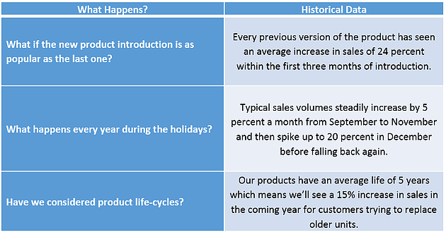
In the end, it’s about mitigating or reducing the impact of purchasing too much too soon. Whilst it makes sense that members of the supply chain want to capture business, it also makes sense that they wait to ensure that the demand is consistent. Granted, it’s much easier said than done. However, by adopting supply chain analytics that rely upon historical data, then companies may be able to better define the seriousness of the increase in demand.