I think it’s important, whatever stage you are at in your career, that you maintain the skills to undertake the analysis, interpretation and presentation of data.
This is especially true for me as an independent supply chain consultant, where the solutions to problems are often established through analytical assessment and modelling.
Personally I actively enjoy the detail and the process of making complex information meaningful and clear for my clients. Consequently I have always kept my MS Excel skills honed. I think MS Excel is probably one of the most powerful business tools introduced since the desktop computer. I’m not sure what businesses did before MS Excel, but probably a lot fewer questions were answered correctly.
Anyway, here’s some basic little MS Excel tricks I’ve picked up along the way. Feel free to comment and share any tips and tricks that you’ve picked up.
1. Flashfill
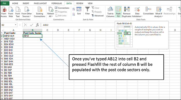
Flashfill is a brilliant new function in MS Excel 2013. To understand how Flashfill works consider that you have a long list of postcodes and you want to extract only the post code sector from the list e.g. for B21 3TH you want to extract the B21 part only. In previous versions of Excel you would have to either use the ‘Text to Columns’ function or write a formula using a range of text formulas i.e. =LEFT, =LEN, =RIGHT etc. Both of these methods could be troublesome especially when the data you wanted to extract was in varying positions in the text string or of varying text lengths.
Flashfill resolves this and makes the task very simple. All you need to do is enter the text you want to extract in the first cell, then hit Flashfill and it will complete the action on all the other field entries for you.
2. Using the ‘TRANSPOSE’ formula (as opposed to using Copy > Paste > Transpose)
So, imagine you have a table of information like the one below that you would like turn 90 degrees.
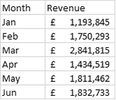
…and you would like the information to be presented as:
The common method to make this change is to use the ‘Paste Special – Transpose’ method. However, this method means that your tables will not be linked. So any changes you make in Table 1 will not be replicated in Table 2. The solution to this is to use the TRANSPOSE formula within an array.
Firstly highlight the cells where you want the new table to appear. Remember that if your original table is 2 columns and 7 rows and you want to turn it 90 degrees, then you will now need to select 2 rows and 7 columns.
When you have selected the cells use the formula bar to select the formula =TRANSPOSE() and then select all the cells in the table your are transposing from.
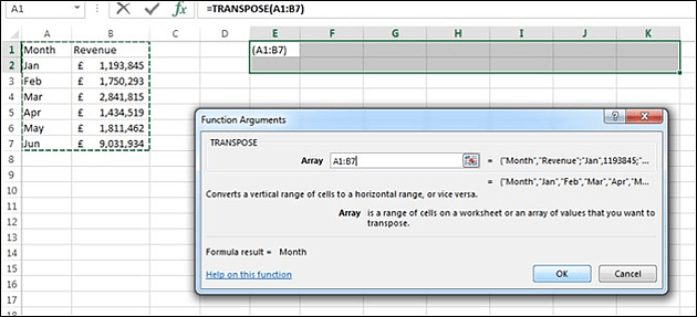
Now, before you click OK you need to turn this into an Array formula. You do this by pressing CTRL and SHIFT at the same time as you click OK.
![]()
3. The ‘Go To Special’ command
Have you ever filtered data and wanted to copy and paste only the data filtered? It’s simple, select the data and press Control and G together. This brings up the ‘Go To’ dialogue box. Click on the button that says ‘Special’ and you will get the options box below.
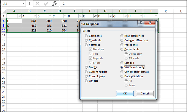
Select the option ‘Visible Cells Only’, press OK and then press Control and C together to copy the information. Now you are able to paste only the filtered information.
Another part of the Go To Special function I find useful is it allows you to highlight only cells with formulas. This in turn allows you to go to Format > Cells > Protection and only protect cells that have formulas. This is particularly useful when you are circulating a spreadsheet to colleagues but you want to restrict their access to formulas.